This release implements the Disney sheen model, which adds two new parameters: sheen and sheenTint. This model adds a new diffuse lobe that attempts to model clothing and textile materials. The effect is subtle but noticeable.
Below we can see the effect of interpolating sheen and sheenTint between 0 to 1 respectively.
We also added the new parameters to our debug visualization system.
Interpolating incoming direction
The effect of sheen tint
Modeling cloth geometry
We made the cloth model in Blender with these steps:
Create a subdivided, one-sided plane surface.
Apply cloth simulation with self-collision turned on.
Freeze the simulation into a static mesh.
Apply smooth shading.
Apply solidify modifier to turn the cloth surface into a two-sided surface with non-zero thickness. We need to do this because Raydiance does not support two-sided surfaces.
Expanding on the skylight model post, we have also made all material properties in a scene tweenable with keyframes. The title video animates multiple material properties and sky model properties simultaneously.
In each video below, we interpolate one material property from 0 to 1 while keeping other parameters the same. In this release, we also exposed specular and specularTint parameters, previously hardcoded as 0.5 and 0, respectively.
Disney model bug fix
We fixed how the specular parameter worked in our Disney BRDF implementation. Previously, sliding the specular parameter between 0 to 1 barely changed the material's appearance, while in the Disney paper, the amount of reflection goes to 0 as the specular goes to 0. The problem was in mixing diffuse and specular BRDFs: we only accounted for the metallic parameter. Unsurprisingly, this bug meant that the specular parameter did not significantly influence the material's appearance. After the fix, our implementation looks better now that we account for metallic and specular parameters.
Additionally, we added the specularTint parameter, which tints incident specular towards the base color. It's intended for additional artistic control.
We have released the skylight model from the previous post as a standalone crate named hw-skymodel. The implementation is almost identical, except that the new() function returns Result instead of assert!.
Publishing into crates.io was straightforward; we had to get an API key and fill in all the required fields in the Cargo.toml file, as mentioned in this article.
This release implements a new skylight model, tone mapping, and a simple
keyframe animation system. This release also unifies all visualization systems
under a single set of tools.
Hosek-Wilkie skylight model
Our previous lighting was a straightforward ad-hoc directional light which we
defined as:
In this release, we replaced it with An Analytic Model for Full Spectral
Sky-Dome Radiance by Lukas Hosek and Alexander Wilkie. This paper
proposes a physically-based analytical model for dynamic daytime skydomes. We
can now animate the sun's position in real-time and have the model produce
realistic sunsets.
The authors wrote a brute-force path tracing simulation for gathering reference
data on atmospheric scattering. They used this reference data to create the
following model.
LλLMλF(θ,γ)χ(H,γ)γθA,B,...,I=spectral radiance=F(θ,γ)⋅LMλ=expected value of spectral radiance=(1+Aecosθ+0.01B)(C+DeEγ+Fcos2γ+Gχ(H,γ)+Icos21θ)=(1+H2−2Hcosα)231+cos2γ=angle between view and sun directions=angle between view and the zenith=model parameters
To evaluate the model, we query the model parameters A,B,...,I and
LMλ from the datasets provided by the authors. Since our renderer
only supports RGB, we must use their RGB datasets.
The sky model runs fast enough to be interactive. Here's a short real-time
demonstration:
Implementation details
The original implementation is implemented ~1000 lines of ANSI C. We could have
built it into our Rust project, but we realized that most of the code was
useless. We re-implemented the original C version into Rust with the following
changes:
We removed spectral and CIE XYZ data sets since our renderer only support
RGB.
We removed the solar radiance functionality since its API only supported
spectral radiances. However, having a solar disc increases realism, so we
might have to revisit this later.
We removed the "Alien World" functionality since we are only concerned with
terrestrial skies.
We switched from double-precision to single-precision computations and
storage. Reduced precision did not seem to have any visual impact and
performed better than doubles.
The model state size went down from 1088 bytes to only 120 bytes.
With these changes, our implementation ended up being just ~200 LOC of Rust.
Simple exposure control
With the new skylight model, we now have a problem: the scene is too bright. We
can scale the brightness down by a constant factor called exposure, which we
are going to define as:
exposure=2stops1,stops≥0
We apply this scaling to every pixel as the final step of the render.
Tone mapping
Dim scene
Bright scene
We can make the image "pop" more with tone mapping, which is a technique for
mapping high-dynamic range (HDR) images into low-dynamic range (LDR) to be shown
on a display device. Our implementation uses the "ACES Filmic Tone Mapping
Curve," which is currently the default tone mapping curve in Unreal Engine. More
specifically, we used Krzysztof Narkowicz's simple curve fit, which
seemed simple, fast enough, and visually pleasing.
We can see in the log plot that the ACES curve boosts colors between 0.1 and
0.7, and then it starts to gracefully dim colors from 0.7 to 10.0. In
contrast, the linear curve clips from 1.0 onwards.
New sky dome visualizations
Elevation between 0..90∘
Turbidity between 1..10
Building on BRDF visualizations from the previous posts, we can also visualize
the sky dome under different parameter combinations.
Offline rendering improvements
The offline rendering mode from the previous post gained some improvements:
Parameters now support simple keyframe animations. Instead of hard-coding
animations like the swinging camera in previous posts, users can now define
keyframes for all sky model parameters. We will continue to expand the number
of animateable parameters in the future, such as object transforms and
material properties.
Offline renders can now have the same text annotations as the BRDF and the new
skydome visualizations.
We also reviewed all our existing visualization systems and combined their
different capabilities under a single set of tools.
The raytracer can now run "offline," which means that we never start up the
Vulkan rasterizer, and the program exits after rendering finishes. This mode can
generate offline rendered animations at high sample counts. The title animation
contains 60 frames, each rendered at 256 samples per pixel.
Raytracer is now multithreaded with rayon. We split the image into
16x16 pixel tiles and use into_par_iter() to render tiles in parallel. On AMD
Ryzen 5950X processor, we can render the cube scene at 66 MRays/s, up from 4.6
MRays/s we had previously with our single-threaded raytracer. If we only used
one sample per pixel, it would run slightly over 60 fps. Of course, the image
would be very noisy, but at least it would be interactive.
To retain our previous single-threaded debugging capabilities, we can set
RAYON_NUM_THREADS=1 to force rayon only to use one thread.
With multithreading, there is a subtle issue with our current random number
generator because we can no longer share the same RNG across all threads without
locking. We can sidestep the whole problem because we can initialize the RNG
with a unique seed at each pixel, like so:
seed=(pixelx+pixely∗imagewidth)∗sampleindex
Multiplying by sampleindex ensures the seed is different at each sample.
With this strategy, we assume that the cost of creating an RNG is negligible
compared to the rest of the raytracer, which is true with rand_pcg.
A popular way to model physically based reflective surfaces is to imagine that
such surfaces are built of small perfect mirrors called microfacets.
Conceptually, each facet has a random height and orientation. The randomness of
these properties determines the roughness of the microsurface. These microfacets
are so tiny that they can be modeled with functions, as opposed to being modeled
with geometry or with normal maps, for example.
D(ωm) is the normal distribution function, or NDF. It describes how
microfacet varies related to the microsurface normal ωm. Disney model
uses the widely popular GGX distribution, so that is what we are
going to use as well.
F(ωi,ωm) describes how much light is reflected from a microfacet.
We use the same Schlick's approximation as we did with Disney diffuse BRDF.
G(ωi,ωo,ωm) is the masking-shadowing function. It
describes the ratio of masked or shadowed microfacets when viewed from a pair of
incoming and outgoing directions. We implemented Smith's height-correlated
masking-shadowing function from this great paper by Eric Heitz called
Understanding the Masking-Shadowing Function in Microfacet-Based
BRDFs.
Microfacet models in practice
What happens if we use a wrong coordinate system
Translating math into source code has a couple of gotchas we need to be aware
of:
Different papers have different naming conventions (incoming vs. light,
outgoing vs. view), and different coordinate systems (z is up vs. y is up),
which can quickly get confusing if we are not being consistent.
Floating point inaccuracies can make various terms go to ∞ or become a
Not a Number. For example, if the incident or outgoing rays are close
to being perpendicular to the surface normal, the cosine of their angles
related to the surface normal approaches zero. Then, any expression divided by
this value results in ∞. The program won't crash, but the image will
slowly become more and more corrupted with black or white pixels. We must take
extra care to clamp such values to a small positive number to avoid dividing
by zero.
Sometimes the sampled vector appears below the hemisphere. In these cases, we
discard the whole sample because those samples have zero reflectance.
We also use the trick from pbrt where they perform all BRDF calculations in a
local space, where the surface normal ωg=(0,1,0). In this local space,
many computations simplify a lot. For example, computing the dot product between
a vector against the surface normal is simply the y-component of the vector. We
can use the same orthonormal basis from the previous posts to go from world to
local space, and once we are done with all BRDF math, we can transform the
results back to world space.
Integrating microfacets with Disney diffuse BRDF
The new specular BRDF introduced three new parameters to our material:
metallic is a linear blend between 0=dielectric and 1=metallic. The
"specular color" is derived from the base color.
specular replaces the explicit index of refraction. It is currently fixed to
0.5 because we don't have a way to get it from GLB yet.
anisotropic defines the degree of anisotropy. Controls the aspect ratio of
the specular highlight. It's currently disabled because our model does not
have tangents.
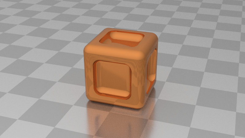
The Disney paper states that their model allows their artists to blend between
any two combinations of parameters and have good results. In the example we
interpolate metallic from 0 to 0.5 to 1.
We now have an interesting problem: choosing which BRDF to sample from. The
Disney paper doesn't describe a method for it, so in our implementation, we draw
a new random variable that selects between diffuse and specular BRDF based on
the metallic parameter. For example, if the metallic value is 0.5, both
diffuse and specular BRDFs are equally likely to be chosen.
Animated BRDF visualizations
Fixed incoming direction Roughness interpolates between 0 and 1
Incoming direction interpolates along x-axis Fixed roughness to 0.25
We dramatically improved the capabilities of the sample placement visualizer
from the previous post. The visualizations are now animated and can render
different text for each frame, and reflectance is directly visualized separately
from probability density functions.
The animations are encoded in APNG format. We chose APNG because:
GIF is too low quality due to limited 256-color palette limitation
WebP's crate takes very long to build and has slightly worse support than APNG
Traditional video formats are not as convenient for short looping animations
rayon for simple data-parallelism to speed up animation renders.
A simple interactive material editor
Having to recompile the program or exporting a new scene from Blender every time
we needed to change the roughness or metallic value quickly became a significant
bottleneck. Since our raytracing is already progressive, we can quickly
implement simple material edits and have the raytracer re-render the image at
each change.
We will rewrite this utility after a more extensive user interface overhaul.
Visualizing normals
Raytraced
Rasterized
While hunting for bugs in our specular BRDFs, we added a simple way to visualize
shading normals in raytraced and rasterized scenes. We will add visualizations
for texture coordinates and tangents in the future.
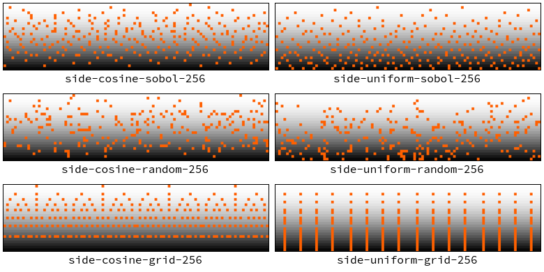
Importance sampling Disney specular models is more challenging than our current
diffuse models. To improve our chances, we created a small tool that visualizes
where the samples are placed around the hemisphere.
We used our existing uniform and cosine-weighted hemisphere samplers to ensure
the tool worked. We also added two additional sample sequences for comparison:
grid sequence, which uniformly samples the unit square.
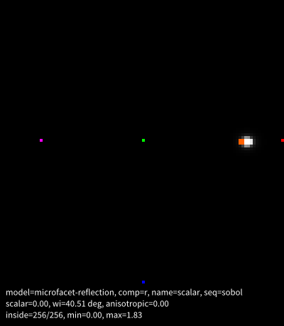
In terms of coordinate spaces, the top plots view the hemisphere from above in
cartesian space. The side plots in x=ϕ=[0,2π] and
y=θ=[0,2π] hemispherical space.
For both sets of plots, the background brightness corresponds to the magnitude
of cosθ.
Looking at the plots, we can intuitively say that cosine performs better than
uniform sampling because it places samples closer to the bright spots.
Similarly, sobol performs better than random and grid.
Note that the new sequences are not currently available for rendering. We will
revisit low-discrepancy sequences later.
Disney principled BRDF is a popular physically based reflectance
model developed by Brent Burley et al. at Disney. It is adopted by
Blender, Unreal Engine, Frostbite, and many
other productions. The team at Disney analyzed the MERL BRDF Database
and fit their model based on MERL's empirical measurements. Their goal was to
create an artist-friendly model with as few parameters as possible. These are
the design principles from the course notes:
Intuitive rather than physical parameters should be used.
There should be as few parameters as possible.
Parameters should be zero to one over their plausible range.
Parameters should be allowed to be pushed beyond their plausible range where it makes sense.
All combinations of parameters should be as robust and plausible as possible.
The full Disney model combines multiple scattering models, some of which we need
to become more experienced with. To avoid getting overwhelmed, we will study and
implement one model at a time, starting with the diffuse model fd, which is
defined as:
Disney's diffuse model is a novel empirical model which attempts to solve the
over-darkening that comes from the Lambertian diffuse model. This darkening
happens at grazing angles, i.e., the angle between the incoming and outgoing
light is close to 0. Disney models this by adding a Fresnel
factor, which they approximated with Schlick's
approximation.
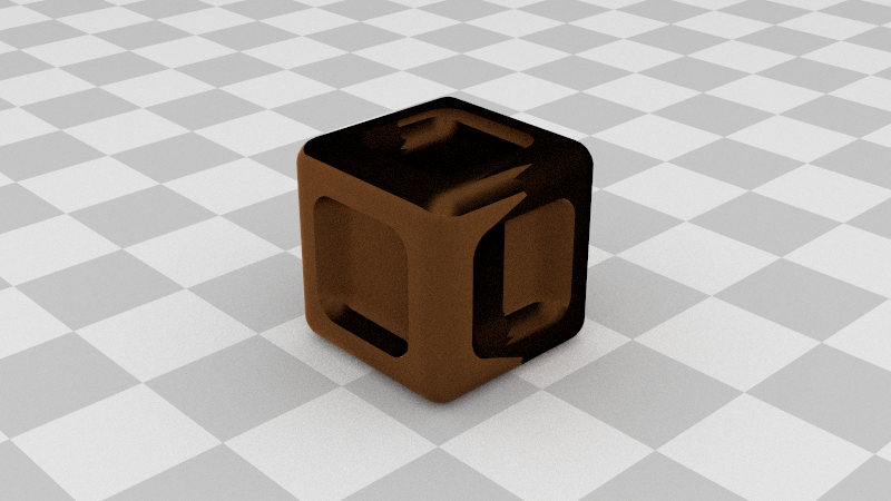
The difference in the comparison above can be subtle. The main difference is
that the cube's edges are slightly brighter compared to the Lambert model, and
the right side of the cube also appears brighter.
Our implementation ignores the "sheen" term and the subsurface scattering
approximation. We will come back to these terms later. Also, any roughness value
below 1 looks incorrect because our current implementation has no specular
terms.
It was time to replace the window title hacks and random keybindings with a real
graphical user interface. We use the the excellent Dear ImGui
library. Since our project is written in Rust, we use imgui and
imgui-winit-support crates to wrap the original
C++ library and interface with winit.
To get a clearer picture, we could increase the number of samples, which would
increase render times, forcing us to find ways to make the renderer run faster.
Alternatively, we could be smarter at using our limited number of samples. This
way of reducing noise in Monte Carlo simulations is called importance
sampling. One of the most impactful techniques for
our simple diffuse cube scene is cosine-weighted hemisphere sampling. Since the
rendering equation has a cosine term, it makes sense to sample from a similar
distribution. We based our implementation on pbrt.
Uniform sampling
Cosine-weighted sampling
Here is the comparison between uniform sampling. It is clear that with identical
sample counts, cosine-weighted sampling results in a much clearer picture than
uniform sampling. And it does it at an equivalent time.
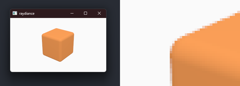
Previously we had to wait until the renderer completed the entire image before
displaying it on the screen. In this commit, we redesigned the path tracing loop
to render progressively and submit intermediate frames as soon as they are
finished. This change significantly improves interactivity.
This commit merges the CPU path tracer with the Vulkan renderer and makes the
camera interactive. As soon as the path tracer finishes rendering, the image is
uploaded to the GPU and rendered on the window. We can also toggle between
raytraced and rasterized images to confirm that both renderers are in sync.
To keep the Vulkan renderer running while the CPU is busy path tracing, we need
to run the path tracer on a separate thread. To communicate across thread
boundaries, we use Rust standard library std::sync::mpsc:channel.
The main thread sends camera transforms to the path tracer, and the path tracer
sends the rendered images back to the main thread. The path tracer thread blocks
the channel to prevent busy looping.
For displaying path traced images on the window, we set up both the uploader and
the rendering pipeline for the image.
We used two tricks to render the image:
To render a fullscreen textured quad, you don't need to create vertex buffers,
set up vertex inputs, etc. With this trick, you can use
gl_VertexIndex intrinsic in the vertex shader to build a huge triangle and
then calculate its UVs. This technique saves a lot of boilerplate code.
In Vulkan, if you want to sample a texture in your fragment shader, you need
to create descriptor pools, and descriptor set layouts, allocate descriptor
sets, make sure pipeline layouts are correct, bind the descriptor sets, and so
on. With VK_KHR_push_descriptor extension, it is possible
to simplify this process significantly. Enabling it allows you to push the
descriptor right before issuing the draw call, saving a lot of boilerplate. We
still have to create one descriptor set layout for the pipeline layout object,
but that is pretty good compared to what we had to do before, only to bind one
texture to a shader.
As a side, vulkan.rs is reaching 2000 LOC, which is getting challenging to
work with. We will have to break it down soon.
The path tracing performance could be better because we are still using only one
thread. It is also why the image is noisier than the previous post since we had
to lower the sample count to get barely interactive frame rates. We will address
the noise and the performance in upcoming commits.
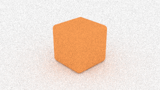
Finally, we are getting into the main feature of raydiance: rendering pretty
images using path tracing. We start with a pure CPU implementation. The plan is
to develop and maintain the CPU version as the reference implementation for the
future GPU version, mainly because it is much easier to work with, especially
when debugging shaders. The Vulkan renderer we've built so far serves as the
visual interface for raydiance, and later, we will use Vulkan's ray tracing
extensions to create the GPU version.
We put this together into a loop, where we bounce rays until they hit the sky or
have bounced too many times. Each pixel in the image does this several times,
averages all the samples, and writes out the final color to the image buffer.
For materials, we start with the simplest one: Lambertian material, which
scatters incoming light equally in all directions. However, a subtle detail in
Lambertian BRDF is that you have to divide the base color with π. Here's the
explanation from pbrt.
For lights, we assume that every ray that bounces off the scene will hit “the
sky.” In that case, we return a bright white color.
For anti-aliasing, we randomly shift the subpixel position of each primary ray
and apply the box filter over the samples. With enough samples, this naturally
resolves into a nice image with no aliasing. pbrt's image
reconstruction chapter has better alternatives for the box filter, which we
might look into later.
We currently run the path tracer in a single CPU thread. This could be better,
but the rendering only takes a couple of seconds for such a tiny image and a low
sample count. We will return to this once we need to make the path tracer run at
interactive speeds.
Currently, raydiance doesn't display the path traced image anywhere. For this
post, we wrote the image out directly into the disk. We will fix this soon.
Implementing MSAA was easy. Similarly to the depth buffer, we create a new color
buffer which will be multisampled. The depth buffer is also updated to support
multisampling. Then we update all the resolve* fields in
VkRenderingAttachmentInfo, and finally, we add the multisampling
state to our pipeline. No more jagged edges.
A lot has happened since our single hardcoded triangle. We can now render
shaded, depth tested, transformed, and indexed triangle lists with perspective
projection.
Loading and rendering GLTF scenes
We created a simple "cube on a plane" scene in Blender. Each object has a
"Principled BSDF" material attached to it. This material is well supported by
Blender's GLTF exporter, which is what we will use for our
application. GLTF supports text formats, but we will export the scene in binary
(.glb) for efficiency.
To load the .glb file, we use gltf crate. Immediately after
loading, we pick out the interesting fields (cameras, meshes, materials) and
convert them into our internal data format. We designed this
internal format to be easy to upload to the GPU. We also do aggressive
validation to catch any properties that we don't support yet, such as textures,
meshes that do not have normals, etc. Our internal formats represent matrices
and vectors with types from nalgebra crate. To turn our
internal formats into byte slices, we use the bytemuck
crate.
Before we can render, we need to upload geometry data to the GPU. We assume the
number of meshes is much less than 4096 (on most Windows hosts, the
maxMemoryAllocationCount is 4096). This assumption allows us to
cheat and allocate buffers for each mesh. The better way to handle allocations
is to make a few large allocations and sub-allocate within those, which we can
do ourselves or use a library like VulkanMemoryAllocator. We will come
back to memory allocators in the future.
To render, we will have to work out the perspective projection, the view
transform, and object transforms from GLTF. We also add a rotation transform to
animate the cube. We pre-multiply all transforms and upload the final matrix to
the vertex shader using push constants. We also pack the base
color into the push constant. Push constants are great for small data because we
can avoid the following:
Descriptor set layouts, descriptor pools, descriptor sets
Uniform buffers, which would have to be double buffered to avoid pipeline stalls
Synchronizing updates to uniform buffers
As a side, while looking into push constants, we learned about
VK_KHR_push_descriptor. This extension could simplify
working with Vulkan, which is exciting. We will return to it once we get into
texture mapping.
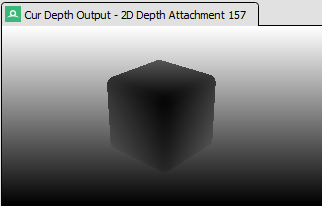
Depth testing with VK_KHR_dynamic_rendering
Depth testing requires a depth texture, which we create at startup, and
re-create when the window changes size. To enable depth testing with
VK_KHR_dynamic_rendering, we had to extend our graphics pipeline with a new
structure called VkPipelineRenderingCreateInfo and add a
color blend state which was previously left out. One additional pipeline barrier
was required to transition the depth texture for rendering.
This is the simplest triangle example rendered without any device memory
allocations. The triangle is hardcoded in the vertex shader, and we index into
its attributes with vertex index.
We added a simple shader compiling step in build.rs which builds
.glsl source code into .spv binary format using Google's glslc,
which is included in LunarG's Vulkan SDK.
Creates semaphores and fences for host-to-host and host-to-device
synchronization.
Clears the screen with a different color for every frame.
We also handle tricky situations, such as the user resizing the window and
minimizing the window.
We don't have to create render passes or framebuffers, thanks to the
VK_KHR_dynamic_rendering extension. However, we have to specify some render
pass parameters when we record command buffers, but reducing the number of API
abstractions simplifies the implementation. We used this
example by Sascha Willems as a reference.
We wrote everything under the main() with minimal abstractions and liberal use
of the unsafe keyword. We will do a semantic compression pass later
once we learn more about how to structure the program.
Next we will continue with more Vulkan code to get a triangle on the screen.
Before anything interesting can happen, we need a window to draw on. We use the
winit crate for windowing and handling inputs. For convenience,
we bound the Escape key to close the window and center the window in the middle
of the primary monitor.
For simple logging, we use log and
env_logger, and for application-level error handling, we
use anyhow.
Next, we will slog through a huge Vulkan boilerplate to draw something on our
blank window.


 What happens if we use a wrong coordinate system

 Fixed incoming direction
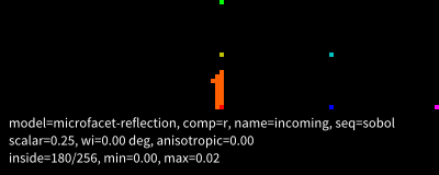 Incoming direction interpolates along x-axis
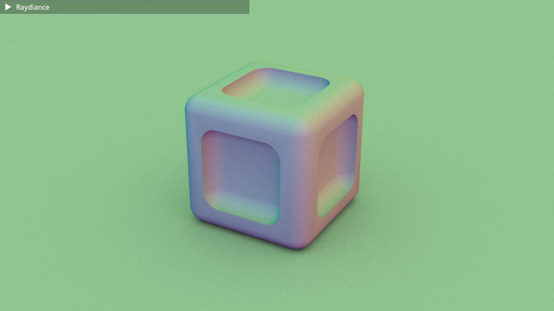 Raytraced
 Rasterized